Loss functions for Deep Learning

This post covers the most common loss functions used in deep learning. Loss functions can be classified as tailored for regression, classification and ranking, based on the specific problem they are designed to address.

Regression

Common regression loss functions include Mean Squared Error (MSE), Mean Absolute Error (MAE) and Huber loss. The SmoothL1Loss implementation in PyTorch is a generalisation of the Huber loss.

Mean Squared Error - L2 loss (MSE) is the default loss for regression problems.

It heavily punishes the model for making large mistakes, and therefore it is not robust to outliers or skewed distributions.

import torch
import torch.nn as nn

#pytorch version
l2_loss = nn.MSELoss()

#custom implementation
def custom_l2_loss(prediction, target):
   return torch.mean((prediction - target)**2)

Mean Absolute Error - L1 loss (MAE) applies less penalty than MSE to heavy losses and tends to produce predictions closer to the median. It is more robust to outliers.

#pytorch version
l1_loss = nn.L1Loss()

#custom implementation
def custom_l1_loss(prediction, target):
    return torch.mean(torch.abs(prediction - target))

The Huber loss offers a compromise between the robustness of MAE and the smoothness of MSE.

#pytorch version
smooth_l1_loss = nn.SmoothL1Loss(beta=1)

#custom implementation
def custom_smooth_l1_loss(prediction, target, beta=1.0):
    diff = torch.abs(prediction - target)
    loss = torch.where(diff < beta, 0.5 * diff**2 / beta, diff - 0.5 * beta)
    return torch.mean(loss)

The SmoothL1Loss implementation with beta = 1 is equivalent to the Huber loss. The transition between the L1 (linear) and L2 (quadratic) parts is controlled by the beta scalar.

If a custom weighting is used, for regression models the weights are applied per data point. Custom weighting may be a good solution to use when tackling skewed distributions, but using too extreme a weighting can lead to instability in the optimizer step due to the variable norms of the weight*gradient for different batches.

Classification

Cross Entropy and its variations are commonly used as loss functions in classification problems.

For each point x and predicted probabilities y , with x representing the one-hot encoding of the true label and y_i representing the predicted probability the point belongs to class i, Cross entropy loss is defined as

\(l(x,y) = - \sum_{i\in C} x_i\log(y_i).\)

Many classification problems tend to have imbalance between the class distribution. For such cases, there are variations of Cross Entropy that can help mitigate the imbalance problems. They give higher weights to smaller classes, and lower weights to the more common classes. Focal Loss and Cross Entropy with Weights are the most commonly used ones.

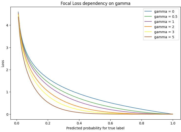
Focal Loss is a special case of Cross Entropy that introduces a term that over-weights hard to predict examples. Keeping same notation as above, focal loss is defined as​

\(l(x,y) = - \sum_{i\in C} x_i (1-y_i)^\gamma\log(y_i) .\)

The parameter gamma controls how certain the model should be before making a prediction. For gamma = 0, we retrieve the original Cross Entropy loss. In the plot below we see that as gamma increases, the model is required to be less certain about a point’s prediction to reach a similar loss. In other words, riskier (less common) predictions are less penalized for larger values of gamma.

PyTorch does not have a built-in class for Focal Loss. Keeping notation similar to other Cross Entropy PyTorch modules, we can define it as below.

import torch
import torch.nn as nn
import torch.nn.functional as F

class FocalLoss(nn.Module):
    def __init__(self, gamma=2, weight=None, reduction='mean'):
        super(FocalLoss, self).__init__()
        self.gamma = gamma
        self.weight = weight
        self.reduction = reduction

    def forward(self, input, target):
        ce_loss = F.cross_entropy(input, target, reduction='none', weight=self.weight)
        pt = torch.exp(-ce_loss)
        focal_loss = (1 - pt) ** self.gamma * ce_loss

        if self.reduction == 'mean':
            return focal_loss.mean()
        elif self.reduction == 'sum':
            return focal_loss.sum()
        else:
            return focal_loss

In the Cross Entropy with Weights loss for each data point is multiplied by the weight associated with its true class.

\(l(x,y) = - \sum_{i\in C} w_i x_i\log(y_i).\)

We can directly use the PyTorch Cross Entropy class and pass it the class weights.

import torch
import torch.nn as nn

# Example weights for three classes
class_weights = torch.tensor([1.0, 2.0, 1.5])  
criterion = nn.CrossEntropyLoss(weight=class_weights)

The use of Focal Loss and Cross Entropy with Weights depends on the level of imbalance in the data, and the resources available for hyperparameter tuning. Finding good weights is a form of hyperparameter search, and generally more sensitive than the choice of gamma in Focal Loss.

Ranking

In the simplest case where the elements to be ranked are considered independently, they can be ranked directly based on a predicted score associated to criteria relevant for the ranking task. In this case, the learning is limited to that of the model for predicting the score and the sorting is independent of the scores for other elements. This method is referred to as pointwise ranking.

Ranking losses that take into consideration inter-element relations can be classified as pairwise or listwise.

Pairwise loss algorithms consider pairs of elements and aim to minimise the number of inversions in ranking the pairs. They transform the ranking problem into a classification or regression formulation. The most popular pairwise ranking algorithms are RankNet, and its variations LambdaNet and LambdaMART.

RankNet example

Given a pair of items (i, j), the goal is to score i higher than j if the ground truth indicates i should be ranked higher than j.

More specifically:

• The network produces prediction scores si, sj for a pair (i, j)

• These are fed into a softmax to produce probability pi that item i should be ranked higher than item j

• If the ground truth has i > j in ranking, we want pi > pj

• Cross-entropy loss is calculated using the ground truth probability q (where q equals 1 if i > j, else 0)

---

Item 1 - Prediction Score s1 = 0.7
Item 2 - Prediction Score s2 = 0.3

Ground Truth Order: Item 1 ranked higher than Item 2

Steps:

1. Feed scores into softmax to get probability p1 that Item 1 ranked higher: p1 = exp(0.7) / (exp(0.7) + exp(0.3)) = 0.668

2. Get p2 for Item 2 ranked higher as 1 - p1 = 0.332

3. Ground truth probability q is 1 since Item 1 ranked higher

4. Cross entropy loss = (-q) * log(p1) - (1-q) * log (p2)

   = (-1) * log(0.668) - 0 * log(0.332)
= 0.403

   ---

So the higher probability assigned to the higher ranked Item 1, the lower our RankNet loss is for this pair. By minimizing this cross-entropy loss across many pairs, the network learns to assign higher scores to items that should be ranked higher per the ground truth.

Listwise algorithms directly consider the entire list of elements and aim to come up with an ordering of it. They work as direct information criteria optimisations (eg. AdaRank) or by minimising a loss defined on specific properties of the kind of ranking to be achieved (eg. ListNet). They tend to be more difficult to train than pointwise o pairwise methods.

Similarity Learning

Contrastive loss is typically used with pairs of samples. It is used in problems where we want similar instances to have embedding that are close in feature space, and dissimilar instances to be far apart in feature space.

For each pair, it computes the distance between the embeddings and adjusts the loss based on whether the pair is similar or dissimilar.

The loss is typically defined as

\(L(y, d) = (1 - y) \cdot d^2 + y \cdot \max(0, m - d)^2 \text{, where } d=dist(x_1,x_2)\)

and y is a binary label similarity indicator (0 for similar pairs, 1 for dissimilar), d is the distance between the embeddings x1 and x2, and m is a margin hyperparameter that represents the minimum desired distance between similar pairs.

Contrastive loss is best suited for data that can be meaningfully represented as pairs, and displays clear characteristics of similarity/dissimilarity. Examples of such problems are metric learning or embedding learning or fine-tuning.

import torch
import torch.nn as nn
import torch.nn.functional as F

class ContrastiveLoss(nn.Module):
    def __init__(self, margin=1.0):
        super(ContrastiveLoss, self).__init__()
        self.margin = margin

    def forward(self, embedding1, embedding2, label):
        distance = F.pairwise_distance(embedding1, embedding2)
        loss = torch.mean((1-label) * torch.pow(distance, 2) +
                          (label) * torch.pow(torch.clamp(self.margin - distance, min=0.0), 2))

        return loss

# Example usage
embedding1 = torch.randn(256)
embedding2 = torch.randn(256)
label = torch.randint(0, 2, (1,)).float()

criterion = ContrastiveLoss(margin=1.0)
loss = criterion(embedding1, embedding2, label)
print("Contrastive Loss:", loss.item())

A special extension of contrastive loss occurs in embedding distillation. Instead of the strict binary labels, it uses continuous labels representing the target similarity degree between two embeddings. These can be obtained from the teacher network. The distillation loss then tries to get embeddings to match these soft similarity targets in the space. Closer targets mean a pair is more contextually related. Embedding distillation retains the overall objective of score-based context learning, but uses continuous rather than discrete labels.

Triplet loss works with triplets of instances, considering the relationship between an anchor, positive, and negative instance. It aims to ensure that the distance between an anchor instance and a positive instance (similar instance) is smaller than the distance between the anchor and a negative instance (dissimilar instance) by a certain margin.

It is usually defined as

\(L(a, p, n) = \max(0, d(a, p) - d(a, n) + m) \)

where a, p, and n represent the anchor, positive, and negative instances, respectively, and m is a margin hyperparameter.

As the formula suggests, distances in the positive cluster are only changed if there is interference from a negative cluster. Here positive and negative are defined relative to the label of the anchor.

Illustration of Triplet loss Schroff et al. 2015

During the training process, it is essential to sample difficult triplets to for the model to learn from. In practice, sampling is done online.

import torch
import torch.nn as nn
import torch.nn.functional as F

class TripletLoss(nn.Module):
    def __init__(self, margin=1.0):
        super(TripletLoss, self).__init__()
        self.margin = margin

    def forward(self, anchor, positive, negative):
        dist_pos = F.pairwise_distance(anchor, positive)
        dist_neg = F.pairwise_distance(anchor, negative)      
        loss = torch.mean(F.relu(dist_pos - dist_neg + self.margin))

        return loss


# Example usage
embedding_size = 256

# Generate dummy data for demonstration
anchor = torch.randn(32, embedding_size)
positive = torch.randn(32, embedding_size)
negative = torch.randn(32, embedding_size)

# Create labels (1 for similar pair, 0 for dissimilar pair)
label = torch.randint(0, 2, (32,)).float()

# Initialize the TripletLoss and calculate loss
criterion = TripletLoss(margin=1.0)
loss = criterion(anchor, positive, negative)
print("Triplet Loss:", loss.item())

The methods presented in this post are by no means comprehensive, but should serve as an introduction to the domain of losses for deep learning.